Pass Your Microsoft Excel Certification Easy!
Microsoft Excel Certification Exams Questions & Answers, Accurate & Verified By IT Experts
Instant Download, Free Fast Updates, 99.6% Pass Rate.
Microsoft Excel Certification Exams Screenshots


Microsoft Excel Product Reviews
Download Free Microsoft Excel Practice Test Questions VCE Files
| Exam | Title | Files |
|---|---|---|
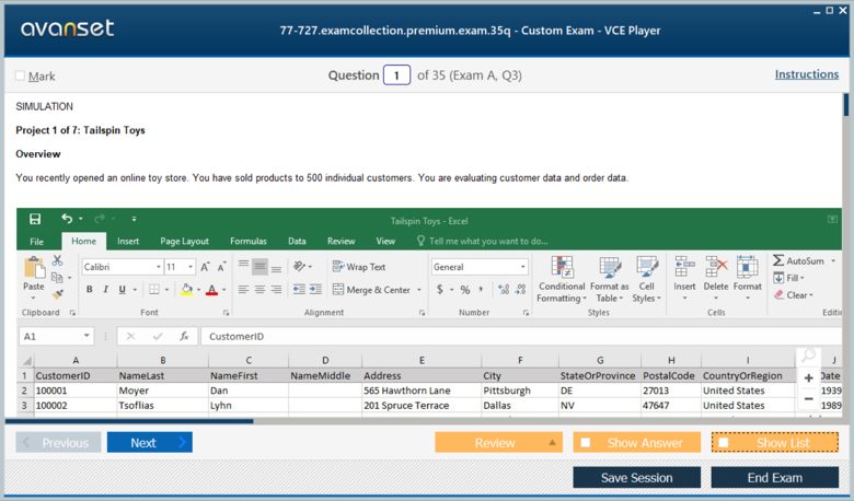
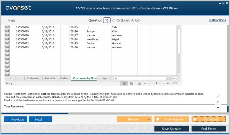
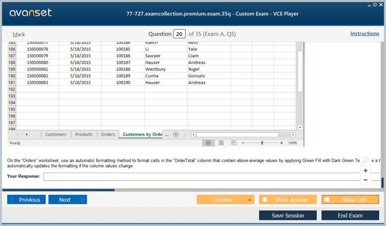
Exam 77-727 |
Title Excel 2016: Core Data Analysis, Manipulation, and Presentation |
Files 2 |
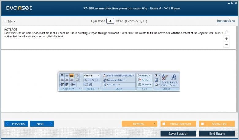
Exam 77-888 |
Title Excel 2010 Expert |
Files 12 |
Microsoft Excel Certification Exam Dumps & Practice Test Questions
Prepare with top-notch Microsoft Excel certification practice test questions and answers, vce exam dumps, study guide, video training course from ExamCollection. All Microsoft Excel certification exam dumps & practice test questions and answers are uploaded by users who have passed the exam themselves and formatted them into vce file format.
Mastering Professional Excellence: The Complete Guide to Microsoft Excel Certifications
In today's data-driven business environment, proficiency in Microsoft Excel has transcended from a desirable skill to an indispensable requirement across virtually every industry. The exponential growth of data analytics, financial modeling, and business intelligence has created an unprecedented demand for professionals who can harness Excel's sophisticated capabilities to drive organizational success. This comprehensive guide explores the intricate landscape of Microsoft Excel certifications, providing you with the essential knowledge needed to make informed decisions about your professional development trajectory.
The modern workplace has undergone a dramatic transformation, with organizations increasingly relying on data-driven insights to maintain competitive advantages. From multinational corporations to emerging startups, businesses across all sectors recognize that professionals equipped with advanced Excel skills possess the ability to streamline operations, enhance productivity, and generate substantial cost savings. Excel certifications serve as tangible proof of these capabilities, distinguishing qualified candidates in an increasingly competitive job market.
Understanding the nuances of different certification pathways, preparation strategies, and career implications requires careful consideration of multiple factors. This extensive guide delves deep into every aspect of Excel certification, from foundational concepts to advanced specializations, ensuring you possess the comprehensive knowledge necessary to select the most appropriate certification path for your unique career aspirations.
The evolution of Excel from a simple spreadsheet application to a powerful business intelligence tool has created diverse opportunities for professionals seeking to validate their expertise. Whether you're an aspiring data analyst looking to establish credibility, a seasoned finance professional aiming to advance your career, or a business manager seeking to optimize operational efficiency, the right Excel certification can serve as a catalyst for professional growth and increased earning potential.
Revolutionary Impact of Excel Certifications on Modern Career Trajectories
The contemporary business landscape demands professionals who can navigate complex data environments with confidence and precision. Microsoft Excel certifications have emerged as critical differentiators in this competitive ecosystem, providing individuals with the credentials necessary to demonstrate their analytical capabilities and technical proficiency to potential employers and stakeholders.
Excel certification programs have undergone significant evolution since their inception, transforming from basic competency assessments to comprehensive evaluations of advanced analytical skills. Today's certification frameworks assess candidates' abilities to perform sophisticated data manipulation, create complex financial models, develop automated reporting systems, and implement business intelligence solutions that drive organizational decision-making processes.
The demand for certified Excel professionals has surged across numerous industries, reflecting the growing recognition of data literacy as a fundamental business skill. Financial services organizations seek certified professionals who can construct intricate risk assessment models and perform complex scenario analyses. Healthcare institutions require certified Excel experts to manage patient data, conduct epidemiological studies, and optimize resource allocation. Manufacturing companies depend on certified professionals to implement supply chain analytics, quality control metrics, and operational efficiency measurements.
Human resources departments increasingly prioritize candidates with verified Excel expertise, understanding that these individuals can contribute immediately to data-driven initiatives without requiring extensive additional training. The certification serves as a reliable indicator of problem-solving capabilities, attention to detail, and commitment to professional excellence that extends far beyond technical proficiency.
Research conducted by leading workforce analytics firms indicates that professionals holding Excel certifications experience significantly faster career advancement compared to their non-certified counterparts. These individuals demonstrate higher levels of job satisfaction, increased responsibility delegation, and greater involvement in strategic decision-making processes. The certification validates not only technical competence but also the analytical mindset essential for thriving in data-centric roles.
The globalization of business operations has further amplified the value of Excel certifications, as organizations seek professionals capable of managing multinational datasets, conducting cross-cultural analyses, and implementing standardized reporting frameworks across diverse geographical locations. Certified professionals possess the credibility necessary to lead international projects, collaborate with global teams, and ensure consistency in analytical methodologies across organizational boundaries.
Excel certification holders often find themselves positioned as internal consultants, called upon to solve complex business challenges, optimize existing processes, and develop innovative solutions that enhance organizational performance. This elevated positioning frequently translates to increased visibility within organizations, expanded networking opportunities, and accelerated career progression trajectories that might otherwise require years of experience to achieve.
Comprehensive Analysis of Certification Benefits and Professional Advantages
The decision to pursue Excel certification represents a strategic investment in long-term career development that yields multifaceted returns across various professional dimensions. Understanding these comprehensive benefits enables individuals to make informed decisions about certification timing, pathway selection, and preparation strategies that align with their specific career objectives and industry requirements.
Enhanced marketability constitutes one of the most immediate and tangible benefits of Excel certification. Certified professionals distinguish themselves in applicant pools through verified competency demonstration, reducing hiring managers' uncertainty about candidate capabilities. This competitive advantage becomes particularly pronounced in industries where data analysis, financial modeling, and reporting accuracy are paramount to organizational success.
The financial implications of Excel certification extend well beyond initial salary negotiations, encompassing long-term earning potential, promotion opportunities, and career mobility options. Salary benchmark studies consistently demonstrate that certified Excel professionals command premium compensation packages compared to their non-certified peers, with salary differentials ranging from fifteen to twenty-five percent depending on industry sector and geographical location.
Professional credibility enhancement represents another significant certification benefit, particularly for individuals transitioning between industries or seeking to establish expertise in new functional areas. The certification provides objective validation of skills that might otherwise require extensive portfolio development or lengthy probationary periods to demonstrate. This credibility acceleration proves invaluable for consultants, freelancers, and entrepreneurs seeking to establish client confidence quickly.
Skill development acceleration through structured certification preparation often reveals advanced Excel features and methodologies that professionals might never encounter through casual usage or informal training. The comprehensive curriculum coverage ensures systematic exposure to sophisticated functionality, optimization techniques, and best practices that enhance overall analytical capabilities beyond immediate certification requirements.
Networking opportunities within professional certification communities provide access to industry experts, thought leaders, and fellow practitioners who share similar career interests and challenges. These connections often facilitate knowledge exchange, collaboration opportunities, and career advancement prospects that extend far beyond the certification achievement itself.
Organizational impact amplification occurs when certified professionals apply their enhanced skills to existing business challenges, often generating measurable improvements in efficiency, accuracy, and decision-making quality. These contributions elevate professional standing within organizations, increase project assignment opportunities, and demonstrate tangible value that supports advancement requests and compensation negotiations.
Continuous learning motivation fostered by certification achievement often inspires professionals to pursue additional credentials, expand their analytical toolkit, and maintain currency with evolving technology trends. This growth mindset becomes increasingly valuable as organizations seek adaptable professionals capable of embracing emerging tools and methodologies without extensive retraining investments.
Strategic Framework for Certification Selection and Career Alignment
Selecting the appropriate Excel certification pathway requires careful evaluation of multiple variables including current skill level, career objectives, industry requirements, time availability, and financial considerations. This strategic framework provides a systematic approach to certification decision-making that maximizes professional development return on investment while minimizing opportunity costs and preparation challenges.
Current competency assessment serves as the foundation for certification selection, requiring honest evaluation of existing Excel knowledge, practical application experience, and familiarity with advanced features. Individuals comfortable with basic formulas, data entry, and simple formatting might benefit from foundational certification programs that provide comprehensive skill building opportunities. Conversely, professionals already utilizing pivot tables, advanced functions, and macro development should consider advanced certifications that recognize and expand upon existing expertise.
Career trajectory analysis involves examining target positions, industry trends, and organizational requirements to identify certification pathways that align with professional aspirations. Data analyst roles typically require advanced statistical function knowledge and data visualization capabilities, while financial positions emphasize modeling expertise and scenario analysis proficiency. Project management roles might prioritize template development, collaborative features, and reporting standardization skills.
Industry-specific requirements vary significantly across sectors, with some emphasizing particular Excel capabilities over others. Healthcare organizations might prioritize data privacy compliance and regulatory reporting features, while manufacturing companies focus on quality control metrics and operational dashboards. Understanding these sector-specific emphases ensures certification selection aligns with relevant industry demands.
Time investment considerations encompass both preparation duration and ongoing maintenance requirements associated with different certification levels. Entry-level certifications typically require fewer preparation hours but may necessitate eventual advancement to remain competitive. Advanced certifications demand substantial initial investment but provide longer-lasting credibility and recognition within professional communities.
Financial planning extends beyond examination fees to include preparation materials, training courses, potential lost productivity during study periods, and opportunity costs associated with alternative skill development options. Comprehensive cost-benefit analysis should consider both immediate expenses and long-term financial returns associated with certification achievement.
Learning style compatibility assessment helps identify preparation methodologies that optimize retention and performance outcomes. Visual learners might benefit from video-based training programs and interactive demonstrations, while kinesthetic learners prefer hands-on practice exercises and simulation-based preparation. Understanding personal learning preferences enhances preparation efficiency and examination performance probability.
Professional development integration ensures certification pursuit complements existing career advancement activities rather than competing with other priorities. Successful professionals often coordinate certification timing with performance review cycles, project completion milestones, or industry conference schedules to maximize visibility and career impact opportunities.
Mastering Fundamental Excel Skills Through Entry-Level Certification Programs
Entry-level Excel certification programs provide comprehensive foundation building for professionals seeking to establish credible expertise in spreadsheet applications and data management fundamentals. These programs typically focus on essential operational competencies that form the cornerstone of more advanced analytical capabilities, ensuring participants develop solid technical foundations while gaining confidence in Excel's primary functionality.
Data entry and formatting mastery represents a critical component of foundational certification programs, encompassing proper cell reference techniques, data validation implementation, and consistent formatting application across complex workbooks. Participants learn to maintain data integrity through structured input methodologies, implement error-checking procedures, and establish formatting standards that enhance readability and professional presentation quality.
Formula construction and basic function utilization form the analytical foundation upon which advanced Excel capabilities are built. Entry-level programs emphasize mathematical operations, logical functions, text manipulation techniques, and date calculations that support routine business operations. Participants master relative and absolute referencing concepts, understand function syntax requirements, and develop troubleshooting skills necessary for formula debugging and optimization.
Worksheet management and organization skills ensure participants can create, maintain, and navigate complex workbooks efficiently. These competencies include sheet naming conventions, tab organization strategies, cell protection implementation, and workspace customization techniques that enhance productivity and reduce errors in multi-worksheet environments.
Basic data visualization through chart creation and formatting enables participants to communicate analytical insights effectively to diverse audiences. Entry-level programs cover chart type selection criteria, data range specification, formatting customization, and integration techniques that support presentation development and stakeholder communication requirements.
Print optimization and document preparation skills ensure participants can produce professional-quality hard copy outputs that meet organizational standards and regulatory requirements. These capabilities include page layout configuration, header and footer customization, scaling adjustment, and quality control procedures that support formal reporting and documentation needs.
Collaboration and sharing functionality introduction provides participants with essential skills for multi-user environments and distributed team collaboration. Entry-level programs address comment integration, change tracking, file sharing protocols, and version control strategies that support effective teamwork and project coordination across diverse organizational structures.
Security and data protection awareness ensures participants understand fundamental safeguarding principles necessary for protecting sensitive information and maintaining compliance with organizational policies. These concepts include password protection implementation, access control understanding, and backup procedures that support data integrity and confidentiality requirements in professional environments.
Advanced Certification Pathways for Sophisticated Data Analysis and Modeling
Advanced Excel certification programs cater to professionals requiring sophisticated analytical capabilities, complex modeling expertise, and comprehensive data manipulation skills that support high-level decision-making processes within organizations. These programs assume foundational competency while focusing on specialized techniques, automation methodologies, and strategic applications that distinguish expert-level practitioners from casual users.
Pivot table mastery and advanced data analysis techniques form the cornerstone of advanced certification programs, enabling participants to transform raw datasets into actionable business intelligence through sophisticated aggregation, filtering, and cross-tabulation methodologies. Advanced practitioners learn to construct dynamic reporting systems, implement conditional formatting rules, and create interactive dashboards that support real-time decision-making processes across organizational hierarchies.
Complex formula development and nested function implementation enable advanced practitioners to construct sophisticated calculations that automate complex business logic and support scenario modeling requirements. These skills encompass array formulas, lookup functions, conditional logic implementation, and error handling techniques that ensure robust analytical solutions capable of handling diverse data conditions and edge cases.
Macro development and automation programming introduce advanced practitioners to Visual Basic for Applications programming concepts that enable process automation, repetitive task elimination, and custom functionality creation. Participants learn to record, edit, and optimize macros while understanding security implications, debugging procedures, and deployment strategies that support enterprise-level automation initiatives.
Data import and integration capabilities enable advanced practitioners to connect Excel with external data sources, including databases, web services, and cloud-based platforms that support comprehensive analytical workflows. These skills encompass connection establishment, data refresh procedures, transformation techniques, and quality assurance protocols that ensure reliable analytical foundations for complex modeling initiatives.
Advanced charting and visualization techniques extend beyond basic graph creation to encompass sophisticated dashboard development, interactive elements, and custom visualization solutions that support executive-level presentations and strategic planning processes. Advanced practitioners master combination charts, dynamic range implementation, and conditional formatting integration that enhances analytical communication effectiveness.
Financial modeling expertise and scenario analysis capabilities enable advanced practitioners to construct comprehensive business models that support strategic planning, investment evaluation, and risk assessment activities. These competencies include sensitivity analysis implementation, Monte Carlo simulation techniques, and optimization procedures that support sophisticated financial analysis and decision support requirements.
Collaboration and enterprise integration skills ensure advanced practitioners can implement Excel solutions within broader organizational technology ecosystems while maintaining security, compliance, and performance standards. These capabilities encompass SharePoint integration, Power Platform connectivity, and enterprise reporting protocols that support scalable analytical solutions across large organizational structures.
Comprehensive Examination Preparation Strategies and Success Methodologies
Effective examination preparation requires systematic approach development that addresses knowledge gaps, builds practical competency, and develops test-taking strategies specifically tailored to Excel certification requirements. Success depends on comprehensive preparation planning, consistent practice implementation, and strategic resource utilization that maximizes learning efficiency while ensuring thorough coverage of examination objectives.
Structured study schedule development forms the foundation of successful certification preparation, requiring realistic timeline establishment, milestone identification, and progress tracking mechanisms that maintain motivation while ensuring comprehensive topic coverage. Effective schedules balance intensive study periods with review sessions, practical application exercises, and rest periods that optimize retention and prevent burnout during extended preparation phases.
Learning resource diversification ensures comprehensive skill development through multiple instructional methodologies that reinforce key concepts and provide varied practice opportunities. Successful candidates typically combine official documentation review, video-based training programs, hands-on practice exercises, and peer discussion forums to create well-rounded preparation experiences that address different learning styles and competency areas.
Practical application emphasis through real-world scenario practice ensures theoretical knowledge translates effectively to practical competency during examination conditions. Preparation activities should include complex problem-solving exercises, time-constrained practice sessions, and scenario-based challenges that mirror actual examination requirements while building confidence and competency in unfamiliar situations.
Knowledge gap identification and targeted remediation enable efficient preparation resource allocation by focusing intensive study efforts on areas requiring improvement while maintaining proficiency in stronger skill areas. Regular self-assessment through practice examinations, skill evaluations, and progress checkpoints helps identify specific topics requiring additional attention and ensures comprehensive preparation coverage.
Test-taking strategy development encompasses time management techniques, question analysis methodologies, and stress management approaches that optimize performance during actual examination conditions. Successful candidates practice examination timing, develop systematic question approach strategies, and implement relaxation techniques that maintain focus and composure throughout extended testing periods.
Performance tracking and adjustment procedures ensure preparation strategies remain effective and responsive to learning progress throughout the study period. Regular evaluation of study effectiveness, retention rates, and practical application success enables preparation plan modifications that optimize learning outcomes while addressing emerging challenges or opportunities for improvement.
Confidence building through graduated challenge progression helps candidates develop psychological readiness for examination pressure while reinforcing technical competency through increasingly complex practice scenarios. Successful preparation programs incorporate confidence-building exercises, positive reinforcement strategies, and success visualization techniques that support optimal performance during high-stakes testing situations.
Industry-Specific Applications and Specialized Career Pathways
Excel certification applications vary significantly across industry sectors, with different professional environments emphasizing specific competencies, analytical approaches, and technical requirements that align with sector-specific business challenges and regulatory environments. Understanding these industry nuances enables targeted certification selection and preparation strategies that maximize career relevance and professional advancement opportunities within chosen sectors.
Financial services organizations demand Excel expertise in areas including risk modeling, portfolio analysis, regulatory reporting, and investment evaluation that require sophisticated mathematical capabilities and precise analytical methodologies. Financial professionals benefit from certifications emphasizing advanced functions, statistical analysis, and scenario modeling techniques that support complex decision-making processes and regulatory compliance requirements specific to banking, insurance, and investment management environments.
Healthcare sector applications focus on patient data management, epidemiological analysis, resource optimization, and quality metrics tracking that require attention to data privacy regulations and clinical accuracy standards. Healthcare professionals pursuing Excel certification should emphasize data validation techniques, compliance reporting capabilities, and analytical methodologies that support evidence-based decision-making while maintaining strict confidentiality and accuracy requirements inherent in medical environments.
Manufacturing and operations environments utilize Excel for supply chain analytics, quality control monitoring, inventory optimization, and production planning that require real-time data integration and process improvement capabilities. Manufacturing professionals benefit from certifications emphasizing automation techniques, dashboard development, and statistical process control methodologies that support lean manufacturing initiatives and continuous improvement programs.
Marketing and sales applications encompass customer relationship management, campaign performance analysis, market research evaluation, and revenue forecasting that require customer data integration and trend analysis capabilities. Marketing professionals pursuing certification should focus on data visualization techniques, customer segmentation methodologies, and performance tracking systems that support data-driven marketing strategy development and campaign optimization.
Human resources departments utilize Excel for workforce analytics, compensation analysis, performance tracking, and compliance reporting that require sensitive data handling and regulatory adherence capabilities. Human resources professionals benefit from certifications emphasizing data protection protocols, statistical analysis techniques, and reporting standardization methodologies that support strategic workforce planning and organizational development initiatives.
Consulting and project management environments require Excel expertise in areas including project tracking, resource allocation, client reporting, and financial modeling that support diverse client requirements and project delivery methodologies. Consulting professionals should pursue certifications emphasizing template development, collaboration features, and presentation integration techniques that enhance client deliverable quality and project management effectiveness.
Research and academic applications focus on data collection, statistical analysis, research documentation, and publication preparation that require academic integrity standards and sophisticated analytical capabilities. Academic professionals pursuing Excel certification should emphasize statistical function mastery, data visualization techniques, and research methodology integration that support scholarly work and publication requirements within academic environments.
Future-Proofing Your Career Through Continuous Learning and Skill Development
The rapidly evolving technology landscape requires Excel professionals to maintain currency with emerging trends, new feature releases, and evolving industry best practices that influence certification relevance and career advancement opportunities. Future-proofing strategies ensure long-term professional value while adapting to changing organizational requirements and technological developments that affect Excel usage and integration within broader business intelligence ecosystems.
Emerging technology integration encompasses understanding how Excel interacts with artificial intelligence platforms, machine learning tools, cloud-based analytics services, and automated reporting systems that are reshaping modern data analysis workflows. Professionals must develop familiarity with Power Platform integration, Microsoft 365 collaboration features, and third-party application programming interfaces that extend Excel functionality beyond traditional spreadsheet applications.
Continuous skill development through ongoing education, professional development courses, and industry conference participation ensures practitioners maintain cutting-edge expertise while building professional networks that support career advancement opportunities. Successful professionals establish learning schedules that incorporate new feature exploration, advanced technique mastery, and industry trend analysis that keeps their capabilities aligned with evolving market demands.
Professional community engagement through user groups, online forums, and industry associations provides access to collective knowledge, emerging best practices, and collaborative learning opportunities that accelerate skill development while building professional relationships. Active community participation often leads to mentorship opportunities, collaboration possibilities, and career advancement prospects that extend beyond individual skill development achievements.
Certification maintenance and advancement planning ensures credentials remain current and relevant while preparing for next-level achievement opportunities that support continued career progression. Many certification programs require periodic renewal, continuing education credits, or advanced level progression that maintains credential value while demonstrating ongoing professional commitment to excellence and skill development.
Cross-functional skill development in related areas including data science, business intelligence, project management, and industry-specific knowledge creates comprehensive professional profiles that distinguish candidates in competitive job markets. Excel expertise combined with complementary skills often creates unique value propositions that support specialized role opportunities and increased earning potential across diverse career pathways.
Strategic Career Planning and the Role of Certification Achievement
In today's dynamic and competitive job market, career success is often not the result of a single leap but rather a series of calculated steps. For professionals looking to elevate their careers, a well-thought-out career plan can be a powerful tool. Within this strategy, certification achievement plays a critical role in enhancing one's skills, marketability, and overall career trajectory. By aligning certification goals with long-term career objectives, industry trends, and organizational advancement opportunities, professionals can strategically position themselves for growth and success.
This article explores the importance of strategic career planning and how certifications—particularly in high-demand fields—are essential in advancing your career. We'll discuss how certifications can be integrated into your career development plans, the benefits of earning a certification, and how to strategically leverage these credentials to achieve career excellence.
The Importance of Aligning Certifications with Career Goals
Strategic career planning is about taking a long-term approach to your professional development. It involves aligning your skills, education, and certifications with the specific career objectives you wish to achieve. One of the most powerful tools in this regard is professional certification, which not only demonstrates your commitment to continual learning but also helps you stand out in a competitive job market.
Certifications are more than just badges of accomplishment. They represent a commitment to mastering skills and knowledge that are highly relevant to the industry and the specific career path you're pursuing. By aligning your certification efforts with your career goals, you ensure that each credential you earn builds on the previous one, forming a cohesive narrative of professional growth.
For example, someone in the IT field looking to advance from a system administrator to a network security expert might plan their certification path to start with basic networking certifications, progressing to more specialized certifications like network security or cloud computing. This strategic alignment ensures that each certification brings the person closer to their long-term career aspirations while making them more attractive to prospective employers.
How Certification Timing Can Maximize Career Advancement
Achieving certifications should not be done in isolation or as a reaction to job demands. Rather, it should be strategically timed to align with key milestones in your career, such as performance reviews, project completions, or planned career transitions. By synchronizing certification achievements with these key events, professionals can make their accomplishments more impactful.
For example, if you know a performance review is coming up or a promotion is on the horizon, acquiring a relevant certification just before these events can provide you with a compelling talking point. It shows your commitment to self-improvement and enhances your qualifications, potentially making you a more valuable candidate for career advancement.
Similarly, timing certification achievements around organizational needs or changes can also be beneficial. For instance, if an organization is transitioning to a new technology platform or system, obtaining a certification relevant to that technology can demonstrate your proactive approach and your ability to contribute to the company's goals.
The Role of Innovation and Creativity in Career Growth
Certifications are not only about acquiring knowledge but also about applying that knowledge creatively. Successful professionals often go beyond the basics by experimenting with new techniques, creating custom solutions, and driving process improvement initiatives. This innovation is essential for career advancement because it demonstrates your ability to think critically and adapt to ever-changing industry requirements.
Excel, for instance, is a tool used across multiple industries, and proficiency in it is highly valued. However, experts in Excel often go beyond standard spreadsheet functions by creating complex formulas, automating tasks with VBA (Visual Basic for Applications), and developing custom solutions for their organizations. This proactive approach to problem-solving distinguishes high-performing professionals from their peers.
By contributing innovative solutions and sharing knowledge with colleagues, individuals not only build a reputation for excellence but also create opportunities for themselves in terms of career advancement and professional recognition. Such contributions often lead to faster promotions and greater professional visibility.
Excel Certification: A Key to Unlocking Career Potential
One of the most widely recognized certifications in today’s business world is Excel certification. Mastery of Excel is crucial for professionals in various roles, from finance and marketing to project management and operations. The ability to manipulate data, create financial models, and visualize insights is highly sought after by employers.
An Excel certification showcases your ability to handle large datasets, create complex formulas, and automate tasks using macros and VBA. However, beyond just technical proficiency, Excel certification reflects your strategic mindset and your capacity to bring greater efficiency to organizational processes.
For many professionals, obtaining Excel certification is a key milestone that can open doors to new career opportunities. Whether it's improving your chances of a promotion or enhancing your qualifications for new job prospects, Excel certification often acts as a differentiator in a crowded job market.
The Benefits of Certification Achievement on Career Development
Earning certifications, whether in Excel or another domain, offers several distinct advantages that significantly impact your professional journey. These include improved job performance, enhanced job security, higher earning potential, and expanded professional opportunities.
1. Increased Job Competence and Performance
Certifications often require professionals to acquire a deep understanding of specific tools, technologies, or methodologies. As such, they foster a higher level of competence in the areas they cover. When you are equipped with the knowledge and skills that certifications validate, you become more effective in your current role. This increased job performance is often noticed by employers and can lead to faster career advancement.
2. Improved Earning Potential
Certified professionals often earn higher salaries than their non-certified counterparts. This is because certifications reflect a higher level of expertise and a commitment to professional growth. Whether you work in IT, marketing, finance, or any other field, certifications tend to have a direct impact on your earning potential. For example, Excel certification can significantly boost your salary as it adds value to your role by improving your efficiency and productivity.
3. Expanded Career Opportunities
Certifications provide a competitive edge, especially in industries where specific skills are in high demand. When you hold a certification, employers are more likely to consider you for job opportunities that align with your qualifications. For professionals in data-driven roles, for example, being Excel certified can give you access to positions that require advanced data analysis, reporting, and visualization skills.
Furthermore, certifications provide opportunities for lateral movement within organizations. For instance, someone with an Excel certification might transition from an administrative or operational role to a more analytical or strategic position, providing greater career satisfaction and growth prospects.
4. Professional Recognition and Credibility
Certifications not only increase your marketability but also build your professional credibility. They demonstrate that you have the skills and knowledge necessary to succeed in your role. For professionals looking to establish themselves as thought leaders or subject matter experts, certifications add authority and legitimacy to their profiles.
Making Strategic Certification Decisions
While certifications are powerful tools for professional development, it is essential to choose the right certifications that align with your career goals. Here’s how you can make informed decisions about which certifications to pursue:
1. Evaluate Industry Trends
Before pursuing a certification, research the current industry trends to understand which skills are in demand. In data-driven environments, for example, certifications in Excel, data analytics, or business intelligence may be more valuable. In cybersecurity, certifications in cloud security or ethical hacking could offer better career prospects.
2. Align Certifications with Career Objectives
Consider how a specific certification fits into your broader career objectives. If your goal is to transition to a leadership role, certifications in project management, leadership, or organizational development might be beneficial. On the other hand, if you aim to become a technical expert, pursuing certifications that validate your expertise in specialized tools or technologies, such as advanced Excel, could be more appropriate.
3. Understand Certification Requirements
Each certification has its own set of requirements, including prerequisites, coursework, or exams. Carefully review these requirements to determine whether the certification aligns with your current level of expertise and whether you have the time and resources to invest in it.
4. Consider Long-Term Value
While it’s tempting to pursue certifications that offer immediate benefits, think about the long-term value of the credential. Does the certification provide transferable skills? Does it have recognition within your industry? Will it open doors for future growth and career advancement?
Maximizing Career Potential through Excel Certification: A Strategic Investment
As businesses become more data-driven, proficiency in tools like Excel has become a pivotal skill that can set professionals apart in today’s competitive job market. While basic Excel skills have long been a requirement in most job descriptions, advanced proficiency, such as advanced formulas, pivot tables, and VBA (Visual Basic for Applications), can significantly elevate one’s career trajectory. Excel certification is not merely a recognition of knowledge but a strategic investment that offers substantial returns in career growth, financial rewards, and professional satisfaction. This article explores how Excel certification provides professionals with a strategic edge and why it’s an essential asset for career development in the modern workforce.
Understanding the Value of Certification in Excel
Certifications serve as proof of expertise in a given field. They communicate to potential employers, clients, and colleagues that a professional has dedicated the time, resources, and effort to mastering a skill or area of knowledge. When it comes to Excel, certification not only showcases your technical capabilities but also signals that you can handle more complex data manipulation tasks, automate processes, and generate insights that guide business decisions. These are highly desirable skills, particularly in data-heavy industries like finance, marketing, operations, and project management.
Unlike traditional degrees or diplomas, Excel certification demonstrates a more hands-on, practical understanding of Excel’s capabilities. It is a testament to the fact that you are not only proficient in basic functionalities but also capable of leveraging the advanced features Excel offers for in-depth analysis and decision-making. This makes Excel certification particularly valuable in roles that require daily data handling, reporting, and visualization tasks.
Boosting Professional Marketability with Excel Certification
In today’s competitive job market, standing out is more challenging than ever before. Many industries and employers have high expectations of their employees, particularly in fields that rely on big data and analytical decision-making. One of the most effective ways to boost your professional profile and increase your marketability is through certification. Excel certification, specifically, serves as a clear demonstration of your ability to handle data at a higher level of expertise.
Excel certification can act as a differentiator on your resume, especially in industries where employers are looking for professionals with advanced Excel skills. Having this certification enhances your chances of securing high-paying roles, including positions like data analyst, business analyst, financial analyst, or project manager. In fact, for professionals already in such positions, Excel certification may act as a springboard for career advancement by showcasing your expertise and readiness for more senior responsibilities.
Moreover, Excel certification provides an immediate demonstration of competency, which is often more impactful than self-reported claims of experience. As employers seek professionals who can drive efficiency and streamline processes, Excel-certified individuals can be seen as assets who contribute to organizational goals in a more immediate and measurable way.
Unlocking Career Growth Opportunities Through Excel Certification
Career growth doesn’t happen by accident. It requires continuous skill development, strategic positioning, and a proactive approach to leveraging industry trends. By achieving an Excel certification, professionals position themselves as more qualified candidates for upward mobility. Whether you're looking for promotions within your current organization or exploring new opportunities in the job market, Excel certification provides a clear path to career advancement.
For professionals already employed in an administrative or operational capacity, Excel certification opens doors to more strategic and analytical roles. For example, someone working as an administrative assistant might use their Excel certification to transition into roles such as data analyst, operations manager, or financial planner. The certification not only expands their skill set but also aligns them with the growing demand for data-driven decision-making in business.
For those already working in managerial or senior roles, Excel certification is a way to stay relevant and competitive in a fast-evolving digital landscape. Senior-level professionals can use the certification to validate their expertise in leading data-driven initiatives or optimizing business processes through advanced data analysis techniques.
Excel Certification’s Impact on Earning Potential
One of the most compelling reasons to invest in Excel certification is its potential to increase earning power. Certification represents a commitment to expertise and self-improvement, and employers are often willing to reward that commitment with higher salaries. Certified professionals are seen as more competent and efficient in their roles, especially when it comes to handling complex data, generating reports, and making data-driven decisions.
In fields like finance, marketing, and project management, where data analysis and reporting are critical, Excel-certified individuals often earn higher salaries than their non-certified counterparts. This is particularly evident in positions that require more advanced Excel skills, such as financial analysts, business intelligence analysts, or data scientists. Excel proficiency can significantly increase your efficiency, which in turn has a direct impact on the bottom line for businesses. As a result, employers are often willing to compensate for this added value.
Moreover, Excel certification can open doors to roles that might not be accessible without it. In highly competitive fields, many job postings require a certain level of Excel proficiency, and having certification ensures that you meet or exceed those expectations. This can provide access to higher-paying opportunities and ensure that you’re compensated fairly for your expertise.
Strengthening Professional Reputation and Credibility
Certification is a tangible way to demonstrate your professional credibility. It provides third-party validation of your skills and can be a powerful tool for building your reputation in your industry. Employers, colleagues, and clients are more likely to trust professionals who have proven their expertise through a recognized certification.
For Excel-certified professionals, this increased credibility can lead to greater recognition within their organizations or industries. Excel proficiency is universally recognized as an essential skill, and being certified allows professionals to establish themselves as experts in their field. This can enhance your reputation not only within your organization but also in broader industry circles, potentially leading to consulting opportunities, networking connections, and speaking engagements.
Additionally, as organizations continue to rely on data to make critical business decisions, the ability to use tools like Excel efficiently becomes more valuable. Professionals who can consistently deliver high-quality, data-driven insights are highly respected, and certification offers a concrete way to establish that expertise.
Certification as Part of a Long-Term Professional Development Plan
For professionals serious about their careers, certifications are not one-time achievements—they are part of a broader, long-term development strategy. In a world where industries, technologies, and business practices are constantly evolving, continuous learning is key to maintaining a competitive edge.
Excel certification can serve as a foundation upon which additional certifications or professional development opportunities are built. For example, an Excel-certified professional might go on to pursue certifications in other business intelligence tools such as Tableau, Power BI, or SQL, further deepening their expertise in data analytics and visualization.
Moreover, certifications can be integrated into performance reviews, project completions, and other career milestones. By strategically planning your certifications in line with your career progression, you ensure that you are always one step ahead of your peers and well-positioned for leadership opportunities.
Conclusion
When considering certification, professionals often wonder about the return on investment (ROI)—how much value they will gain from the time, effort, and resources spent on obtaining it. The ROI on Excel certification can be measured in several ways.
Firstly, Excel-certified professionals tend to enjoy faster career progression. They are often able to take on more complex and impactful projects, leading to quicker promotions and salary increases. Secondly, the demand for Excel expertise continues to grow across industries, making it an asset that doesn’t lose value over time. Whether you are staying with your current employer or moving to a new one, Excel certification is a credential that is universally recognized and respected.
The financial return is also significant. In many industries, Excel certification can boost salaries by as much as 20-30% or more. Over the course of a career, this translates to substantial increases in lifetime earning potential. Even if you are already in a senior position, Excel certification can serve as a valuable tool to maintain your competitive edge and ensure that you continue to advance.
Excel certification is not just about mastering a tool—it’s about demonstrating your ability to leverage data to drive business decisions, improve efficiency, and solve complex problems. This skill is invaluable in the modern job market, where data analysis and decision-making are at the heart of most industries.
As businesses place greater emphasis on data-driven strategies, Excel-certified professionals are in high demand. By pursuing this certification, you gain not only technical skills but also a strategic advantage in your career. From boosting your marketability and enhancing your earning potential to increasing your professional credibility and reputation, the benefits of Excel certification are clear.
Incorporating Excel certification into your long-term career development plan can provide significant returns, both financially and professionally. Whether you’re looking to advance in your current role or open doors to new opportunities, Excel certification is a powerful tool for achieving long-term career success and securing your place as a highly sought-after professional in the marketplace.
ExamCollection provides the complete prep materials in vce files format which include Microsoft Excel certification exam dumps, practice test questions and answers, video training course and study guide which help the exam candidates to pass the exams quickly. Fast updates to Microsoft Excel certification exam dumps, practice test questions and accurate answers vce verified by industry experts are taken from the latest pool of questions.


Microsoft Microsoft Excel Video Courses


Top Microsoft Certifications


Top Microsoft Certification Exams
- AZ-104
- AZ-305
- DP-700
- AB-100
- SC-300
- MD-102
- PL-300
- AB-900
- MS-102
- SC-200
- SC-401
- AI-900
- AZ-900
- AZ-700
- AI-103
- DP-600
- AI-102
- AZ-500
- SC-100
- AB-730
- AB-731
- GH-300
- PL-400
- AZ-140
- AZ-204
- SC-900
- AZ-400
- DP-300
- AZ-801
- MS-700
- AZ-800
- PL-600
- MB-800
- PL-200
- AI-300
- PL-900
- AI-901
- MB-310
- MB-330
- SC-500
- DP-900
- MB-820
- DP-800
- MB-230
- MB-280
- GH-200
- MS-721
- DP-750
- MB-500
- MB-700
- DP-420
- DP-100
- GH-900
- PL-500
- GH-500
- MB-335
- GH-100
- MS-900
- AZ-120
- SC-400
- MB-240
- MO-200
- 62-193
- MO-400
- MS-203
- MB-910
- DP-203
- 98-367
Site Search:


@dimpoz, do not worry pal...u should have used several excel practice tests instead because u cannot rely on one material and expect to pass...otherwise u can do a retake and come out successful....never too late
i regret having visited this site because ms excel prep material that i encountered is so invalid that made me think i was fully prepared yet only 2 questions were familiar....i terribly failed…please, advise…are those available here reliable?
hurrayy!!!i passed the exams but i have one thing which made me perceive this exam to be so easy....excel certification classes are very good since it has all the units that needs to be covered before doing exam
i needed to be part of the excel elites but i cannot manage the microsoft excel certification cost this is too much for me...cant they reduce plz
@zorro, all the microsoft excel prep materials available here are valid to let you pass...plz do not fear using them....they cant mislead you
in order to recognised for ms excel certification u need to pass exams and the only way to pass is using the materials that comrades keep on uploading here.
hey....do not be much stressed the things are easy nowadays....with online excel certification u can have all the materials and exams u need at any time anywhere
who has utilized excel certification test....is it valid for one to totally rely on.
@morris, what i can i advise you to do is to use excel certification course which has all the concepts that are tested in the forthcoming exam
hey comrades....plz use all the materials designed for excel certification because the exams test on all concepts presented during the training
i have just got enrolled to microsoft excel certification program...which is are the best materials to use during the preparation...anyone???